More on HTab Parameters

Written by ironcore | March 9, 2011

I’ve mentioned this a lot in this blog, but I’m finding more and more that a good, solid definition of your HTab parameters up front will go a long way in helping construct a nice stable unsteady flow model in HEC-RAS.

First, let me recap how they work. In unsteady flow, HEC-RAS will convert the geometry of cross sections into a set of curves defining relationships between hydraulic parameters and stage (it does the same thing for bridges and culverts, but we’ll save that for another post). These hydraulic parameters include conveyance, flow area, storage area, and top width. This is done for the main channel, overbanks, and for the total cross section. Storage area in this case represents any ineffective flow areas in the given cross section. The figure below shows the conveyance HTab curve for a cross section.

These curves (actually the paired data that creates them) are used by HEC-RAS during the unsteady flow computations. Rather than re-computing the hydraulic parameters at every time step, RAS can simply pick the value off the chart. Because these curves are defined by a number of discrete points, RAS usually must interpolate to grab a value in between points. RAS does this linearly. Herein lies the problem that can lead your model to errors and instabilities.

Notice how at the lower stages, there is a significant curvature to the conveyance relationship in the above figure? A linear interpolation in this range can be quite wrong if the resolution of points is too coarse. Notice how when I zoom in to a rather coarse Conveyance HTab curve, it becomes obvious that in between points, linear interpolation is going to give me a bad answer. This is why a good definition of HTab points is particularly advantageous when running at low stages.

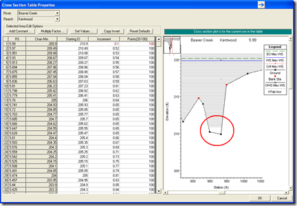
Start by maximizing the number of HTab points for you cross sections. HEC-RAS allows up to 100. The grey horizontal lines in the figure below represent computation points at different stages. I know what you’re thinking. “Won’t that many points on every cross section really slow down the computations?” Well, that may have been the case years ago, but computers are so fast now, that you’ll probably never notice the difference. Furthermore, the development of these curves is only done once, during the preprocessing part of the computations. As long as you don’t change the geometry, RAS won’t have to recompute the HTab curves.

Then make the computation increment as small as possible to squeeze all the points together. You only need to extend your HTab curves to contain the maximum computed water surface.

Finally, go to the Stating El. column and click the button “Copy Invert”. Notice in the figure below there is a gap between the invert of the channel and the first computation point which is set 1 ft above the invert of the main channel.

This is the default starting computation point in RAS (well, not completely true). If you check the 2nd figure up above, you’ll see that there actually was a computation point at the 0 depth point (the invert). That’s because RAS will still compute the 0 depth point, but then the next computation point, by default, is 1 ft (0.3 meters in SI Units) above the 0 depth point. From there on up, RAS will space the computation points based on the increment you define. To get more points between the invert of the main channel and 1 ft (0.3 m) above the invert, you have to set your Starting Elevation to the invert. That’s why it’s always a good idea to click “Copy Invert” and make sure that your Starting Elevation is the same as your “Chan Min” value. That way, the small computation increment is started from the channel invert, not 1 ft (0.3 m) above the channel invert.

I was recently informed that in the next release of HEC-RAS (version 4.2), the default starting point for HTab computations will be 0.5 ft above the invert (0.15 m?). This will improve things somewhat, but it still may be necessary to “copy the invert”, particularly if you have very low stages in your simulation.